20) Parallel Linear Algebra

Last time:

• Introduction to Batch Jobs and Job Scripting

• SLURM Demo

Today:

1. Parallel inner and outer products
   1.1 OpenMP 1.2 MPI

2. Parallel matrix-vector products

1. Parallel inner and outer products

Inner product

For given vectors \(x\) and \(y\), we want to compute their inner (dot) product

\[ x^T y = \sum_{i=1}^N x_i y_i \]

1.1 OpenMP

If we were to use multi-threading via OpenMP, the vectors x and y of length N are stored in a contiguous array in shared memory.

A C snippet would look like the following:

double sum = 0;
#pragma omp parallel for reduction(+:sum)
for (int i=0; i<N; i++)
    sum += x[i] * y[i];

1.2 MPI

If we were to use multi-processing via MPI, the vectors x and y are partitioned into \(P\) parts of length \(n_p\) such that:

\[ N = \sum_{p=1}^P n_p . \]

In the following C snippet the inner product is computed via

double sum = 0;
for (int i=0; i<n; i++)
    sum += x[i] * y[i];
MPI_Allreduce(MPI_IN_PLACE, &sum, 1, MPI_DOUBLE, MPI_SUM, comm);

Things to consider:

• Work: \(2N\) flops processed at a rate \(R\)

• Execution time: \(\frac{2N}{RP} + \text{latency}\)

• How big is latency?

using Plots
default(linewidth=4) # Plots embelishments

P = 10 .^ range(log10(2), log10(1e6), length=100)
N = 1e9         # Length of vectors
R = 10e9 / 8    # (10 GB/s per core) (2 flops/16 bytes) = 10/8 GF/s per core
t1 = 2e-6       # 2 µs message latency

function time_compute(P)
    return 2 * N ./ (R .* P)
end

plot(P, time_compute(P) .+ t1 .* (P .- 1), label="linear", xscale=:log10, yscale=:log10)
plot!(P, time_compute(P) .+ t1 .* 2 .* (sqrt.(P) .- 1), label="2D mesh")
plot!(P, time_compute(P) .+ t1 .* log2.(P), label="hypercube", legend=:bottomleft)
xlabel!("P processors")
ylabel!("Execution time")

Network effects

Remember that we saw a plot from Paul Fischer’s page, researcher at Argonne National Labb and Professor at UIUC, testing different Border Gateway Protocols (BGP).

Here is a different plot comparing “software all_reduce”, meaning traditional MPI based implementation Vs “hardware-accellerated all_reduce”, meaning using GPU-aware MPI:

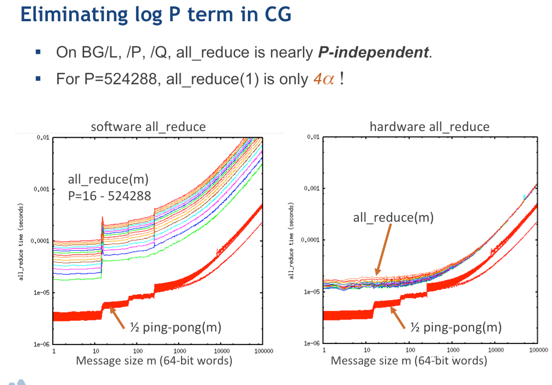
We noticed how the time is basically independent of the number of processes \(P\), and only a small multiple of the cost to send a single message. We attributed this to the good quality of the network.

Torus topology

Networks can be connected with different topologies.

For instance, the torus topology:

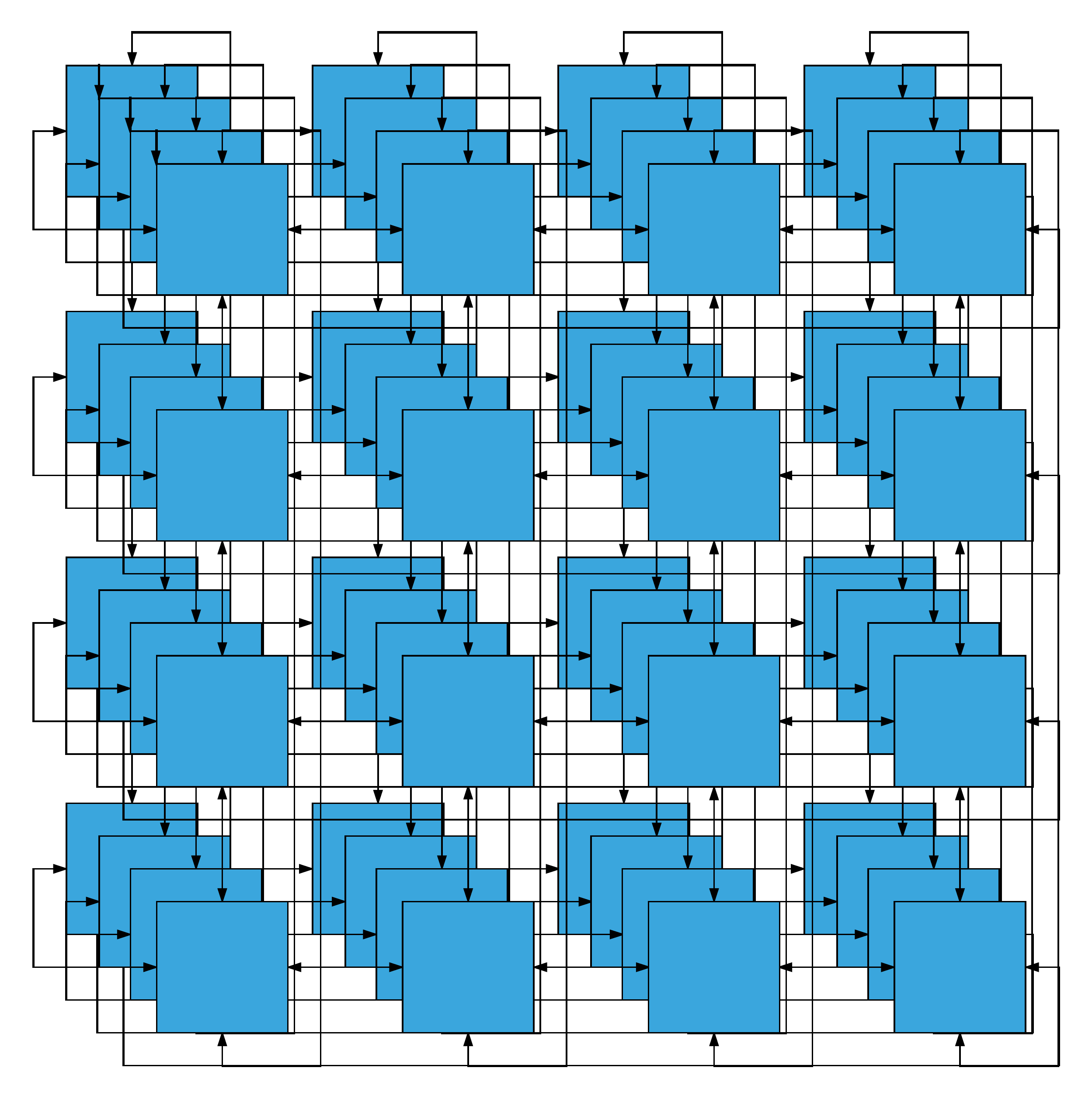
• 3D torus: IBM BlueGene/L (2004) and BlueGene/P (2007)

• 5D torus: IBM BlueGene/Q (2011)

• 6D torus: Fujitsu K computer (2011)

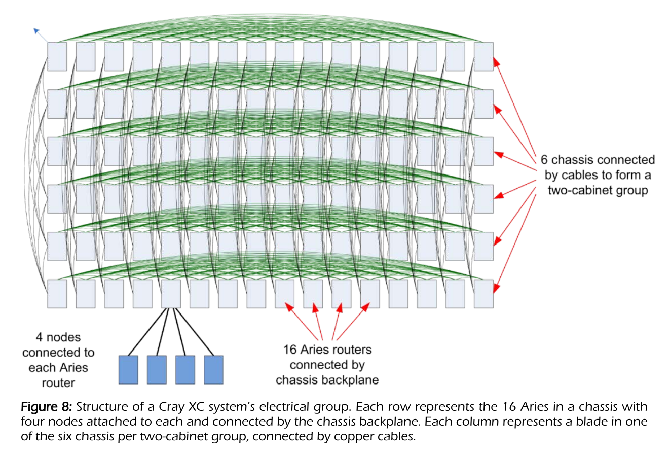
Dragonfly topology

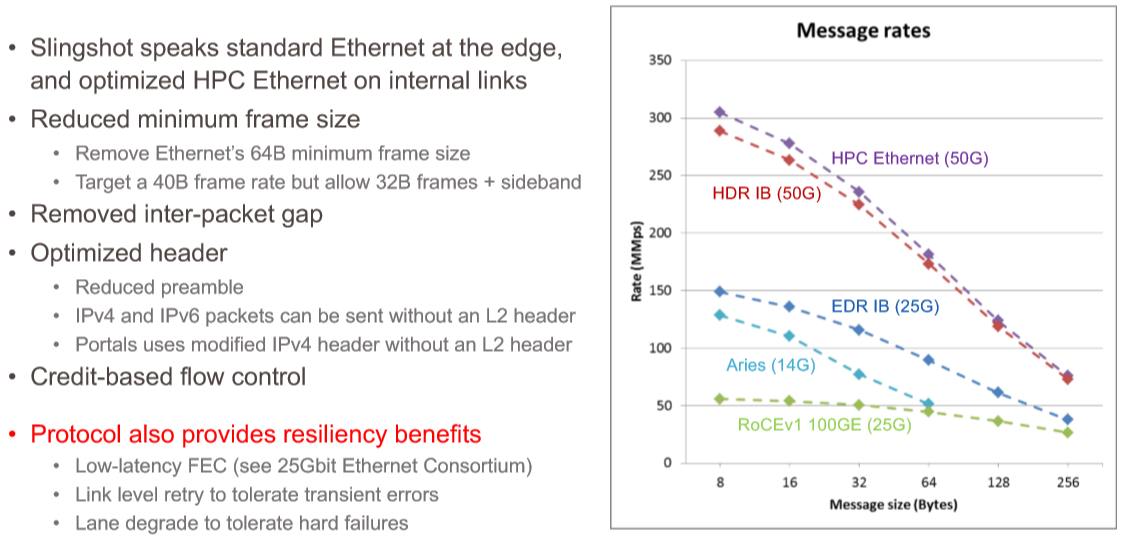
Today’s research: reducing contention and interference

Different vendors might provide different solutions. Here is an example from a few years ago highlighting the capabilities of Cray’s Slingshot network that still illustrates the concept for different protocols and congestion control:

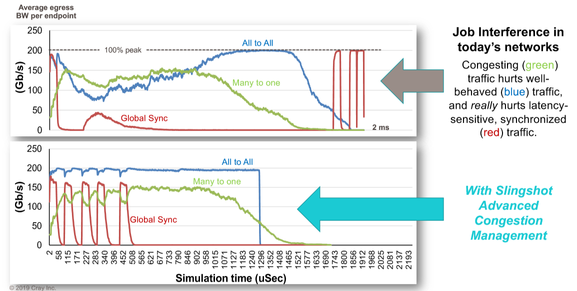
There are three workloads running in the system. The red line is a spikey global synchronization routine, the green one is a many to one collective operation, and the blue one is an all to all scatter operation. This shows Slingshot running with congestion control turned off and then turned on. In the top scenario, the red workload spikes right out of the gate, wildly reduces the blue workload and pulls down the green workload. As they are crashing because of backed up packets, the global synchronization tries to send out another pulse, and it gets stepped on, and it goes totally flat as the blue all to all communication takes over and the green many to one collective finishes up, leaving it some breathing room. Finally, after they are pretty much done, the global synchronization spikes up and down like crazy, finishing its work only because it pretty much as the network to itself. The whole mess takes 2 milliseconds to complete, and no one is happy.

Here is another simulation showing the latency of traces on the network with a bunch of applications running, some of them causing congestion:

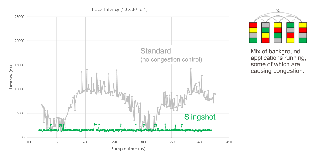
Images from this article.

Compare to BG/Q

• Each job gets an electrically isolated 5D torus

• Excellent performance and reproducibility

• Awkward constraints on job size, lower system utilization.

Outer product

\[ C_{ij} = x_i y_j \]

• Data in: \(2N\)

• Data out: \(N^2\)

2. Parallel matrix-vector products

\[ y_i = \sum_{j} A_{ij} x_j \]

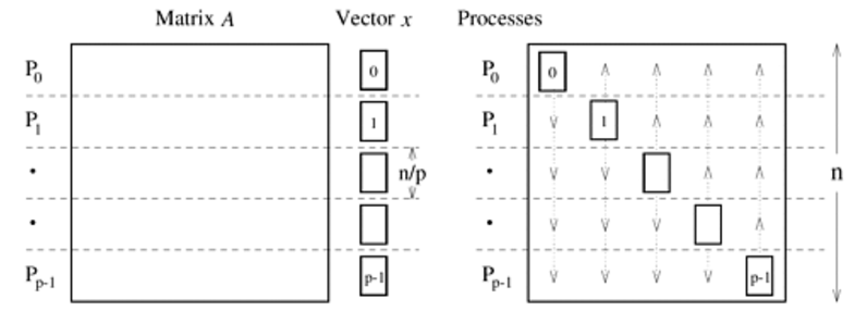
How to partition the matrix \(A\) across \(P\) processors?

1D row partition

• Every process needs entire vector \(x\): MPI_Allgather

• Matrix data does not move

• Execution time

  \[ \underbrace{\frac{2N^2}{RP}}_{\text{compute}} + \underbrace{t_1 \log_2 P}_{\text{latency}} + \underbrace{t_b N \frac{P-1}{P}}_{\text{bandwidth}} \]

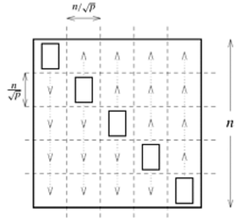
2D partition

• Blocks of size \(N/\sqrt{P}\)

• “diagonal” ranks hold the input vector

• Broadcast \(x\) along columns: MPI_Bcast

• Perform local compute

• Sum y along rows: MPI_Reduce with roots on diagonal

• Execution time

  \[ \underbrace{\frac{2N^2}{RP}}_{\text{compute}} + \underbrace{2 t_1 \log_2 P}_{\text{latency}} + \underbrace{\frac{2 t_b N}{\sqrt{P}}}_{\text{bandwidth}} \]

N = 1e4
tb = 8 * 100 / 1e9 # 8 bytes / (1 GB/s) ~ bandwidth per core in units of double
P = 10 .^ range(log10(2), log10(1e6), length=100)
t1 = 2e-6       # 2 µs message latency

custom_xticks = [10, 100, 1000, 10000, 100000, 1000000]
custom_yticks = [.1, .01, .001, .0001]

plot(P, (2 * N^2) ./ (R .* P) .+ t1 .* log2.(P) .+ tb .* N .* (P .- 1) ./ P, label="1D partition", xscale=:log10, yscale=:log10, xticks=custom_xticks, yticks=custom_yticks, xlims = [2, 1e6])
plot!(P, (2 * N^2) ./ (R .* P) .+ 2 .* t1 .* log2.(P) .+ 2 .* tb .* N ./ sqrt.(P), label="2D partition", xscale=:log10, yscale=:log10, xticks=custom_xticks, yticks=custom_yticks)
xlabel!("P processors")
ylabel!("Execution time")