6) Measuring Performance#
Last time:
Intro to Vectorization
Today:
1. Measuring Performance#
Two of the standard approaches to assessing performance:
Floating Point Operations per Second (FLOP/S)
FLOPs = Floating Pointer Operations (careful on the small “s” vs big “S”) (see video: 1.1.1 GFLOPS).
How many floating point operations (add, subtract, multiply, and maybe divide) a code does per second.
How to estimate: for matrix-matrix multiply we have 2 FLOP per inner loop, and a triply nested loop thus total \(\text{FLOPs} = 2nmk\). The FLOPS are then \(\text{FLOPS} = 2nmk / \text{time}\). Note that usually we use GigaFLOPS or GFLOPS: \(\text{GFLOPS} = 2nmk / \text{time} / 10^9\).
Calculate for one core of your machine:
\[ \text{FLOP/S} = \frac{\text{cycle}}{\text{second}} \frac{\text{FLOPs}}{\text{cycle}} \]cycles-per-second can be looked up for your CPU on your machine
FLOP/S-per-cycle can be tricky to find, is based on your processors microarchitecture and is most easily found on the Wikipedia FLOP page. For instance, consider a laptop with an Intel Core i5-8210Y CPU at 1.6 GHz. This is an Amber Lake processors with 16 FLOPs-per-cycle, and thus has a calculated FLOP rate of
\[ \text{FLOPS} = 1.6 \frac{\text{Gigacycles}}{\text{second}} 16 \frac{\text{FLOPs}}{\text{cycle}} \](Note that some processors support turbo boost so you may see even higher performance unless turbo boost is disabled)
Memory Bandwidth:
Rate at which memory can be moved to semiconductor memory (typically from main memory).
Can be looked up on manufacture page
Measure in Gigabits-per-second (GiB/s) or GigaBytes-per-second (GB/s)
GigaByte (GB): \(1 \text{ GB} = 10^9 \text{ bytes} = 8 \times 10^9 \text{ bits}\)
Gigabit (GiB): \(1 \text{ GiB} = 10^9 \text{ bits}\)
2. Introduction to Performance Modeling#
Models give is a conceptual and roughly quantitative framework by which to answer the following types of questions.
Why is an implementation exhibiting its observed performance?
How will performance change if we:
optimize this component?
buy new hardware? (Which new hardware?)
run a different configuration?
While conceptualizing a new algorithm, what performance can we expect and what will be bottlenecks?
Models are a guide for performance, but not an absolute.
Terms#
Symbol |
Meaning |
|---|---|
\(n\) |
Input parameter related to problem size |
\(W\) |
Amount of work to solve problem \(n\) |
\(T\) |
Execution time |
\(R\) |
Rate at which work is done |
2.1 The vector triad benchmark#
Fathoming the chief performance characteristics of a processor or system is one of the purposes of low-level benchmarking.
A low-level benchmark is a program that tries to test some specific feature of the architecture like, e.g., peak performance or memory bandwidth.
One of the prominent examples is the vector triad, introduced by Schönauer (self-edition, 2000). It comprises a nested loop, the inner level executing a multiply add operation on the elements of three vectors and storing the result in a fourth.
Example in Fortran:#
See the following implementation as a Fortran code snippet:
double precision, dimension(N) :: A,B,C,D
double precision :: S,E,MFLOPS

do i=1,N                                !initialize arrays
    A(i) = 0.d0; B(i) = 1.d0
    C(i) = 2.d0; D(i) = 3.d0
enddo

call get_walltime(S)                    ! get time stamp

do j=1,R
    do i=1,N
        A(i) = B(i) + C(i) * D(i)       ! 3 loads, 1 store
    enddo
    if(A(2).lt.0) call dummy(A,B,C,D)   ! prevent loop interchange
enddo

call get_walltime(E)                    ! get time stamp again

MFLOPS = R*N*2.d0/((E-S)*1.d6)          ! compute MFlop/sec rate
The purpose of this benchmark is to measure the performance of data transfers between memory and arithmetic units of a processor.
On the inner level, three load streams for arrays
B,CandDand one store stream forAare active.Depending on
N, this loop might execute in a very small time, which would be hard to measure. The outer loop thus repeats the triadRtimes so that execution time becomes large enough to be accurately measurable. In practice one would chooseRaccording toNso that the overall execution time stays roughly constant for differentN.
Observations:
The aim of the masked-out call to the
dummy()subroutine is to prevent the compiler from doing an obvious optimization: Without the call, the compiler might discover that the inner loop does not depend at all on the outer loop indexjand drop the outer loop right away.The possible call to
dummy()fools the compiler into believing that the arrays may change between outer loop iterations. This effectively prevents the optimization described, and the additional cost is negligible because the condition is always false (which the compiler does not know in advance).Please note that the most sensible time measure in benchmarking is wallclock time, also called elapsed time. Any other “time” that the system may provide, first and foremost the much stressed CPU time, is prone to misinterpretation because there might be contributions from I/O, context switches, other processes, etc., which CPU time cannot encompass (this is especially true for parallel programs).
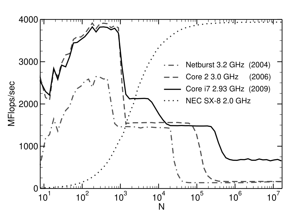
In the above graph, we see the serial vector triad performance versus loop length for several generations of In- tel processor architectures (clock speed and year of introduction is indicated in the legend), and the NEC SX-8 vector processor. Note the entirely different performance characteristics of the latter.
Tip
If you are not familiar, check this reference on How to Compile a C program and How to Compile a Fortran program
2.2 The STREAM benchmark:#
A C snippet:
for (i=0; i<n; i++)
    a[i] = b[i] + scalar*c[i];
Following the notation above, \(n\) is the array size and
is the number of bytes transferred.
The rate \(R = W/T\) is measured in bytes per second (or MB/s, etc.).
Dense matrix multiplication#
To perform the operation \(C \gets C + A B\) where \(A,B,C\) are \(n\times n\) matrices. Again, a C snippet would look like:
for (i=0; i<n; i++)
    for (j=0; j<n; j++)
        for (k=0; k<n; k++)
            c[i*n+j] += a[i*n+k] * b[k*n+j];
Can you identify two expressions for the total amount of work \(W(n)\) and the associated units?
Can you think of a context in which one is better than the other and vice-versa?
Note
C is said to follow the row-major order method.
Fortran, MATLAB, and Julia follow the column-major order method.
If you are not familiar with row/column-major order methods, please see this Wiki page.
Support for multi-dimensional arrays may also be provided by external libraries, which may even support arbitrary orderings, where each dimension has a stride value, and row-major or column-major are just two possible resulting interpretations. For example, row-major order is the default in NumPy (for Python) even though Python itself is neither row or column major (uses lists of lists); Similarly, column-major order is the default in Eigen and Armadillo (libraries for C++).
Estimating time#
To estimate time, we need to know how fast hardware executes flops and moves bytes.
using Pkg
Pkg.add("CSV")
using CSV
Pkg.add("DataFrames")
using DataFrames
Pkg.add("Plots")
using Plots
default(linewidth=4, legendfontsize=12)

hardware = CSV.read("../assets/data/data-intel.csv", DataFrame)
Resolving package versions...
   Installed SentinelArrays ── v1.4.8
   Installed WorkerUtilities ─ v1.6.1
   Installed WeakRefStrings ── v1.4.2
   Installed PooledArrays ──── v1.4.3
   Installed InlineStrings ─── v1.4.5
Installed CSV ───────────── v0.10.15
    Updating `~/.julia/environments/v1.10/Project.toml`
  [336ed68f] + CSV v0.10.15
    Updating `~/.julia/environments/v1.10/Manifest.toml`
  [336ed68f] + CSV v0.10.15
  [48062228] + FilePathsBase v0.9.24
  [842dd82b] + InlineStrings v1.4.5
  [2dfb63ee] + PooledArrays v1.4.3
  [91c51154] + SentinelArrays v1.4.8
  [ea10d353] + WeakRefStrings v1.4.2
  [76eceee3] + WorkerUtilities v1.6.1
Precompiling
packages...
    274.9 ms  ✓ WorkerUtilities
    279.0 ms  ✓ PooledArrays
364.8 ms ✓ InlineStrings
242.3 ms ✓ InlineStrings → ParsersExt
868.2 ms ✓ SentinelArrays
398.3 ms ✓ WeakRefStrings
   5558.3 ms  ✓ CSV
  7 dependencies successfully precompiled in 8 seconds. 314 already precompiled.
Resolving package versions...
Installed InvertedIndices ─ v1.3.1
Installed DataFrames ────── v1.8.0
    Updating `~/.julia/environments/v1.10/Project.toml`
  [a93c6f00] + DataFrames v1.8.0
    Updating `~/.julia/environments/v1.10/Manifest.toml`
  [a93c6f00] + DataFrames v1.8.0
  [41ab1584] + InvertedIndices v1.3.1
Precompiling packages...
227.7 ms ✓ InvertedIndices
17031.0 ms ✓ DataFrames
    744.8 ms  ✓ Latexify → DataFramesExt
  3 dependencies successfully precompiled in 18 seconds. 321 already precompiled.
Resolving package versions...
  No Changes to `~/.julia/environments/v1.10/Project.toml`
  No Changes to `~/.julia/environments/v1.10/Manifest.toml`
| Row | Year | GFLOPs-SP | GFLOPs-DP | Cores | Mem-GBps | TDP | Freq(MHz) | Name |
|---|---|---|---|---|---|---|---|---|
| Int64 | Int64 | Int64 | Int64 | Int64 | Int64 | Int64 | String31 | |
| 1 | 2007 | 102 | 51 | 4 | 26 | 150 | 3200 | Xeon X5482 |
| 2 | 2008 | 108 | 54 | 4 | 26 | 150 | 3400 | Xeon X5492 |
| 3 | 2009 | 106 | 53 | 4 | 32 | 130 | 3300 | Xeon W5590 |
| 4 | 2010 | 160 | 80 | 6 | 32 | 130 | 3300 | Xeon X5680 |
| 5 | 2011 | 166 | 83 | 6 | 32 | 130 | 3470 | Xeon X5690 |
| 6 | 2012 | 372 | 186 | 8 | 51 | 135 | 2900 | Xeon E5-2690 |
| 7 | 2013 | 518 | 259 | 12 | 60 | 130 | 2700 | Xeon E5-2697 v2 |
| 8 | 2014 | 1324 | 662 | 18 | 68 | 145 | 2300 | Xeon E5-2699 v3 |
| 9 | 2015 | 1324 | 662 | 18 | 68 | 145 | 2300 | Xeon E5-2699 v3 |
| 10 | 2016 | 1548 | 774 | 22 | 77 | 145 | 2200 | Xeon E5-2699 v4 |
| 11 | 2017 | 4480 | 2240 | 28 | 120 | 205 | 2500 | Xeon Platinum 8180 |
| 12 | 2018 | 9320 | 4660 | 56 | 175 | 400 | 2600 | Xeon Platinum 9282 |
plot(hardware[:,3], hardware[:,5], xlabel = "GFLOPs Double Precision", ylabel = "Memory GBps", primary=false)
scatter!(hardware[:,3], hardware[:,5], label = "Mem-GBps",)
Here we have rates \(R_f = 4660 \cdot 10^9\) flops/second and \(R_m = 175 \cdot 10^9\) bytes/second. Now we need to characterize some algorithms.
algs = CSV.read("../assets/data/algs.csv", DataFrame)
| Row | Name | bytes | flops |
|---|---|---|---|
| String15 | Int64 | Int64 | |
| 1 | Triad | 24 | 2 |
| 2 | SpMV | 12 | 2 |
| 3 | Stencil27-ideal | 8 | 54 |
| 4 | Stencil27-cache | 24 | 54 |
| 5 | MatFree-FEM | 2376 | 15228 |
Let’s check the operations per byte, or operational intensity:
algs[!, :intensity] .= algs[:,3]  ./ algs[:,2]
algs
| Row | Name | bytes | flops | intensity |
|---|---|---|---|---|
| String15 | Int64 | Int64 | Float64 | |
| 1 | Triad | 24 | 2 | 0.0833333 |
| 2 | SpMV | 12 | 2 | 0.166667 |
| 3 | Stencil27-ideal | 8 | 54 | 6.75 |
| 4 | Stencil27-cache | 24 | 54 | 2.25 |
| 5 | MatFree-FEM | 2376 | 15228 | 6.40909 |
sort!(algs, :intensity)
| Row | Name | bytes | flops | intensity |
|---|---|---|---|---|
| String15 | Int64 | Int64 | Float64 | |
| 1 | Triad | 24 | 2 | 0.0833333 |
| 2 | SpMV | 12 | 2 | 0.166667 |
| 3 | Stencil27-cache | 24 | 54 | 2.25 |
| 4 | MatFree-FEM | 2376 | 15228 | 6.40909 |
| 5 | Stencil27-ideal | 8 | 54 | 6.75 |
function exec_time(machine, alg, n)
    bytes = n * alg.bytes
    flops = n * alg.flops
    machine = DataFrame(machine)
    T_mem = bytes ./ (machine[:, "Mem-GBps"] * 1e9)
    T_flops = flops ./ (machine[:, "GFLOPs-DP"] * 1e9)
    return maximum([T_mem[1], T_flops[1]])
end

Xeon_Platinum_9282 = filter(:Name => ==("Xeon Platinum 9282"), hardware)
SpMV = filter(:Name => ==("SpMV"), algs)

exec_time(Xeon_Platinum_9282, SpMV, 1e8)
0.006857142857142857
pl = plot()
for machine in eachrow(hardware)
    for alg in eachrow(algs)
        ns = exp10.(range(4,9,length=6))
        times = [exec_time(machine, alg, n) for n in ns]
        flops = [alg.flops .* n for n in ns]
        rates = flops ./ times
        plot!(ns, rates, linestyle = :solid, marker = :circle, label="", xscale=:log10, yscale=:log10)
    end
end
xlabel!("n")
ylabel!("rate")
display(pl)
It looks like performance does not depend on problem size.
Well, yeah, we chose a model in which flops and bytes were both proportional to \(n\), and our machine model has no sense of cache hierarchy or latency, so time is also proportional to \(n\). We can divide through by \(n\) and yield a more illuminating plot.
for machine in eachrow(hardware)
    times = [exec_time(machine, alg, 1) for alg in eachrow(algs)]
    rates = algs.flops ./ times
    intensities = algs.intensity
    plot!(intensities, rates, xscale=:log10, yscale=:log10, marker = :o, label = machine.Name, legend = :outertopright)
end

xlabel!("intensity")
ylabel!("rate")
ylims!(1e9, 5e12)
xlims!(5e-2,1e1)
We’re seeing the roofline for the older processors while the newer models are memory bandwidth limited for all of these algorithms.
The flat part of the roof means that performance is compute-bound. The slanted part of the roof means performance is memorybound.
Note that the ridge point (where the diagonal and horizontal roofs meet) offers insight into the computer’s overall performance.
The x-coordinate of the ridge point is the minimum operational intensity required to achieve maximum performance.
If the ridge point is far to the right, then only kernels with very high operational intensity can achieve the maximum performance of that computer.
If it is far to the left, then almost any kernel can potentially hit maximum performance.