9) Packing for cache#
Last time:
Blocked matrix-matrix multiply
Blocking for registers
Optimizing the micro kernel
SIMD.jl
StaticArrays.jl
KernelAbstractions.jl
Today:
In this lecture we are primarily concerned about optimizing the code cache utilization. The big ideas are using a block-block decomposition to target the various levels of cache and repacking the data for more optimal data access in the microkernel.
The most important parts of this are the five loops pictures here:
1. Different levels of cache#
Tip
For this section, watch the video 3.1.1 on the LAFF course to have a basic idea.
As we’ve mentioned previously, there is a hierarchy of memory on modern computers.
Why were these different levels of memory born? The incovenient truth is that floating point computations can be performed very fast while bringing data in from main memory is relatively slow. How slow?
On a typical architecture it takes at least two orders of magnitude more time to bring a floating point number in from main memory than it takes to compute with it.
The physical distance between the CPU and main memory creates a latency for retrieving the data. This could then be offset by retrieving a lot of data simultaneously, increasing bandwidth. Unfortunately there are inherent bandwidth limitations: there are only so many pins that can connect the central processing unit (CPU) with main memory.
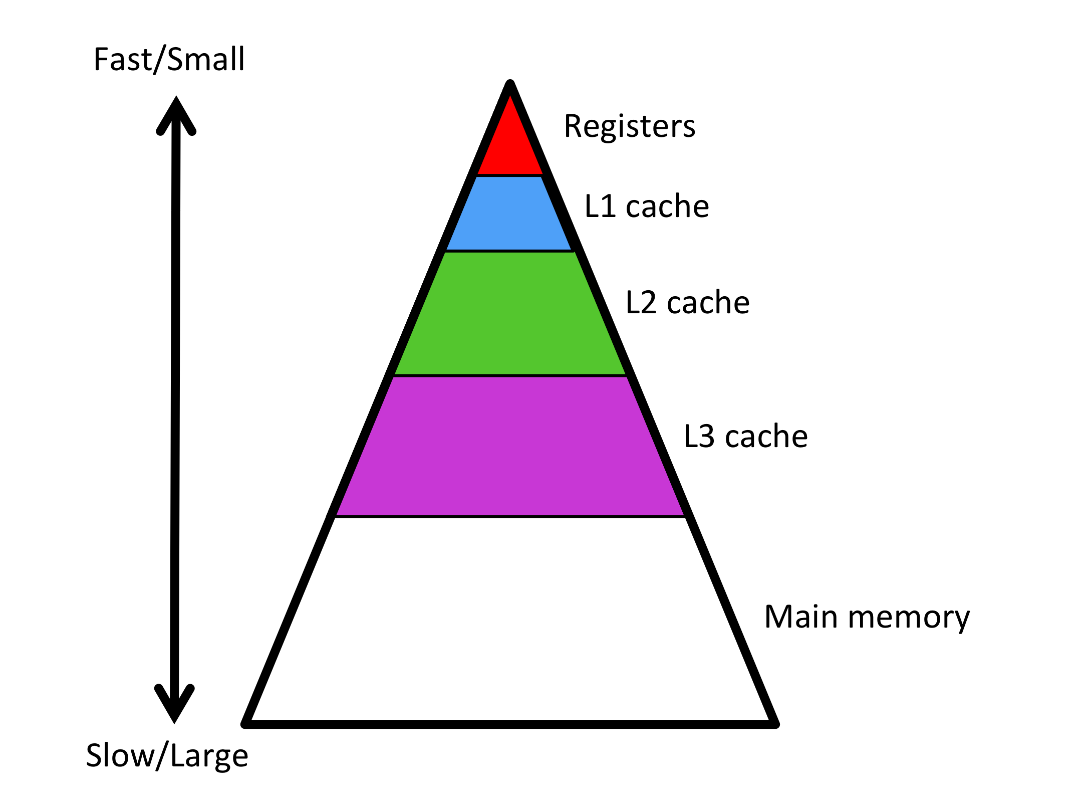
To overcome this limitation, a modern processor has a hierarchy of memories. We have already encountered the two extremes: registers and main memory. In between, there are smaller but faster cache memories. These cache memories are on-chip and hence do not carry the same latency as does main memory and also can achieve greater bandwidth.
How big?
We have:
Registers: ~64
Float64(16 vector registers, each of which can store 4Float64, i.e., double precision floating point values)L1 Cache: ~32 KiB
L2 Cache: ~512 KiB
L3 Cache: ~8 MiB
Main Memory (RAM): ~16GiB
Memory gets smaller and faster as we get closer to the registers (where we can actually compute from). This means that in order to get the most out of our floating point operations we want the data we need to access to be as close to the registers as possible.
What data is in the cache, depends on the cache replacement policy and algorithmically we just want to access the data in a way that encourages the data in the higher caches levels to be used more often.
How big of a matrix fits in these different layers of cache?
Layer |
Size |
Largest \(n \times n\) matrix |
|---|---|---|
Registers |
~16 \(\times\) 4 |
\(n = \sqrt{64} = 8 \Rightarrow 8 \times 8\) matrix |
L1 Cache |
~32 KiB |
\(n = \sqrt{32 \times 1024/8} = 64 \Rightarrow 64 \times 64\) matrix , 4096 |
L2 Cache |
~512 KiB |
\( n = \sqrt{512 \times 1024/8} = 256 \Rightarrow 256 \times 256\) matrix, \(65 526\) |
L3 Cache |
~8 MiB |
\( \sqrt{ 8 \times 1024 \times 1024/8} = 1024 \Rightarrow 1024 \times 1024\) matrix, \( 1 048 576\) |
Main Memory |
~16GiB |
\( \sqrt{ 16 \times 1024 \times 1024 \times 1024/8} = 46341 \Rightarrow 46341 \times 46341\) matrix, 2e9 |
The basic strategy will be to block the matrices into blocks of size \(m_c \times n_c\) for \(C\), \(m_c \times k_c\) for \(A\), and \(k_c \times n_c\) for \(B\) then use the optimized microkernel to compute a single block matrix-matrix multiply.
2. Microkernel and L1 / L2 caches#
Tip
For this section,see the text 3.2 on the LAFF course to have a basic idea.
Remember that we have:
where each block of \(C\) is of size \(m_{b} \times n_{b}\). The matrices \(A\) and \(B\) are partitioned in a conformal manner into \(M \times K\) and \(K \times N\) blocks respectively; the block size associated with \(K\) is \(k_{b}\).
With this partitioning of the matrix, the update for block \(ij\) of \(C\) is then
In the microkernel of last lecture, we had the outer loop ordering:
for j = 1:N
  # micropanel B_j: size kc X nr
  for i = 1:M
    # microtile C_ij: size mr X nr
    # micropanel A_i: size mr X kc

    # call: microkernel: C_ij += A_i * B_j (with any loop ordering)
  end
end
If we chose \(m_b\), \(n_b\), and \(k_b\) such that \(A_{ip}\), \(B_{pj}\) and \(C_{ij}\) all fit in the cache, then we meet our conditions for best performance. We could compute \(C_{ij} = C_{ij} + A_{ip} B_{pj}\), by “bringing these blocks into cache” and computing with them before writing out the result.
The difference here is that while one can explicitly load registers, the movement of data into caches is merely encouraged by careful ordering of the computation, since replacement of data in cache is handled by the hardware, which has some cache replacement policy that will evict the least recently used data.
During last lecture we argued that the \(m_r \times n_r\) microtile of \(C\) should fit in registers, thus \(m_r = 12\) and \(n_r = 4\) were reasonable choices since \(m_r \times n_r = 48\). (We still need some registers for a vector of \(A\) and \(B\) and since we only need one vector register for an element of \(B\), due to the outer product structure (for which we can reuse it), it makes sense that we put more elements in \(m_r\) so that \(m_r \times n_r + m_r + 4 = 64\); (the \(4\) here is the vector register being used for an element of \(B\)).
Poll 9.1: Size \(n\) of largest square (\(n \times n\)) matrices \(A\), \(B\), and \(C\) to fit in L2 (512 KB) cache:#
a) 64
b) 147
c) 442
Now the question is what happens in with the L1 and L2 cache with this loop ordering.
\(A\) and \(B\) are broken into micropanels:
The inner loop of \(I\) means that the \(k_c \times n_r\) micropanel \(B_J\) is fixed for all the micropanels of \(A\). This suggests that we want \(k_c \times n_r\) to fit in the L1 cache so that we got lots of reuse \(B_J\) before having to bring a new micropanel into the L1 cache.
Similarly, since we get to use all of the micropanels of \(A\) when \(J\) is indexed, this suggests we want \(m_c \times k_c\) to fit in the L2 cache.
So to summarize so far:
\(n_r\) and \(m_r\) chosen to fit the microtile of \(C\) in the registers.
\(k_c\) chosen to fit the micropanel of \(B\) in the L1 cache (micropanel of size \(k_c \times n_r\)).
\(m_c\) chosen to fit the block of \(A\) in the L2 cache (block of size \(m_c \times k_c\)).
3. L3 cache#
After the considerations from last lecture, we only have \(n_c\) left to choose, since this impacts the size of the block of \(B\) it makes sense to pick \(k_c \times n_c \) to fit in the L3 cache.
The only question left to answer is then, how to orchestrate loop over the blocks so that we can efficiently use the data block of \(B\) we have placed in the L3 cache and not need to have \(C\) in the cache anywhere?
Namely,
Poll 9.2: which of the loop orderings do we want?#
IJP
IPJ
PIJ
PJI
JPI
JIP
Since we want \(B_{PJ}\) in the L3 cache, this suggests to us that \(I\) should be the inner-most loop, so that once \(B_{PJ}\) is in the cache, it is used completely until expelled, so that this leaves us with only the following two options:
Poll 9.3: which of the following two loop orderings do we want?#
JPI
PJI
If we choose JPI then indexing \(P\) doesn’t impact the choice of block \(C_{IJ}\) which will then imply that data from \(C\) is only loaded once (since the block \(C_{IJ}\) is fully updated before moving onto the next block of \(C\)); however, elements of \(C\) will still have be touched multiple times, since \(C_{IJ}\) is loaded \(M / m_c\) times to do the loop over \(I\).
Q: Should \(m_c \times n_c\) fit in the L3 cache too?
4. Packing#
Tip
Reference text: 3.3 Packing
As we’ve mentioned before, matrices in Julia (and many other applications) are stored with column-major order which means that matrix columns are contiguous in memory. (This is also often referred to as the first index changes the fastest, which is how things get generalized to higher dimensional arrays.)
In the example below notice that the contiguous data is in the columns:
a = zeros(Int, 2, 3)
2×3 Matrix{Int64}:
 0  0  0
 0  0  0
a[:] .= 1:6
6-element view(::Vector{Int64}, :) with eltype Int64:
 1
 2
 3
 4
 5
 6
a[:]
6-element Vector{Int64}:
 1
 2
 3
 4
 5
 6
a
2×3 Matrix{Int64}:
 1  3  5
 2  4  6
This is important because accessing data in the same order it is stored is faster than jumping around; this is all related to vector loads (which we have talked about before) as well as memory pages and cache prefetching.
What does this mean for our code? Two things:
Accessing data along the columns is faster than accessing along the rows
Implication: In the microkernel we access the micropanel \(B\) along rows, which means that we are not getting good caching for the loads
Accessing that next bit of data in the same column is faster than accessing data in a new column (even if the load is a vector load)
Implication: The micropanel of \(A\), which in Julia is a view into the larger \(A\) matrix, is not accessed optimally when we are continuously shifting columns.
Solution: repacking the data into the access pattern we need when we first try to get a submatrix to land in a particular cache (also, if we don’t pack, the submatrices may be in the caches we expect…)
See the BLIS packed 5 loops for the packing we need to implement.