5) Introduction to Vectorization#
Last time:
Introduction to architectures
Memory
Today:
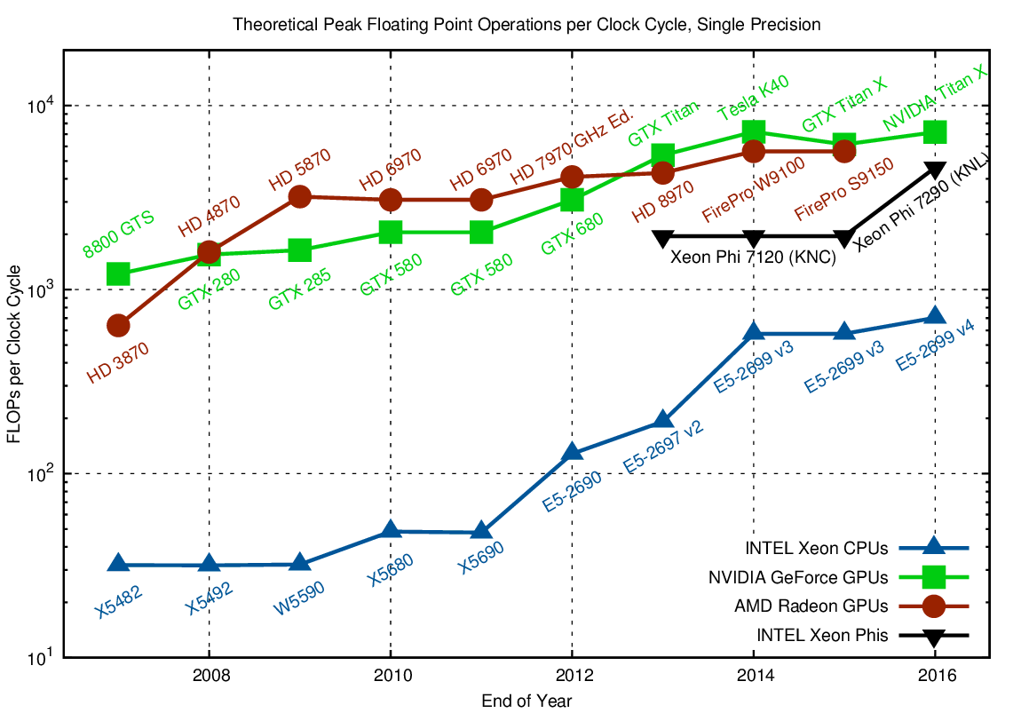
1. Single-thread performance trends#
Single-thread performance has increased significantly since ~2004 when clock frequency stagnated (Moore’s law stopped)?

Source: Microprocessor Trend Data.
How is this possible?
This is a result of doing more per clock cycle.
Further resources#
2. Vectorization#
History: Starting with the Cray 1 supercomputer, vector systems had dominated scientific and technical computing for a long time until powerful RISC-based massively parallel machines became available.
Today, they are part of a niche market for high-end technical computing with extreme demands on memory bandwidth and time to solution.
By design, vector processors show a much better ratio of real application performance to peak performance than standard microprocessors for suitable “vectorizable” code.
They follow the SIMD (Single Instruction Multiple Data) paradigm which demands that a single machine instruction is automatically applied to a — presumably large — number of arguments of the same type, i.e., a vector.
Most modern cache-based microprocessors have adopted some of those ideas in the form of SIMD instruction set extensions.
For vector processors, machine instructions operate on vector registers which can hold a number of arguments, usually between 64 and 256 (double precision).
The width of a vector register is called the vector length, usually denoted by \(L_v\).
Example:#
For getting reasonable performance out of a vector CPU, SIMD-type instructions must be employed.
As a simple example we consider the addition, of two arrays as a Fortran code snippet::
A(1:N)=B(1:N)+C(1:N)
On a cache-based microprocessor this would result in a (possibly software-pipelined) loop over the elements of A, B, and C. For each index, two loads (one for B and one for C), one addition and one store (in the result vector A) operation would have to be executed, together with the required integer and branch logic to perform the loop.
A vector CPU can issue a single instruction for a whole array if it is shorter than the vector register length \(L_v\):
vload V1(1:N) = B(1:N)
vload V2(1:N) = C(1:N)
vadd V3(1:N) = V1(1:N) + V2(1:N)
vstore A(1:N) = V3(1:N)
Here, V1, V2, and V3 denote vector registers.
The distribution of vector indices across the pipeline tracks is automatic. If the array length is larger than the vector length, the loop must be stripmined, i.e., the original arrays are traversed in chunks of the vector length:
do S = 1,N,Lv !  start, stop [,step]
    E = min(N,S+Lv -1)
    L = E-S+1
    vload V1(1:L) = B(S:E)
    vload V2(1:L) = C(S:E)
    vadd V3(1:L) = V1(1:L) + V2(1:L)
    vstore A(S:E) = V3(1:L)
enddo
This is done automatically by the compiler.
An operation like vector addition does not have to wait until its argument vector registers are completely filled but can commence after some initial arguments are available. This feature is called chaining and forms an essential requirement for
different pipes (like MULT and ADD) to operate concurrently.
Writing a program so that the compiler can generate effective SIMD vector instructions is called vectorization.
Sometimes this requires reformulation of code or inserting source code directives in order to help the compiler identify SIMD parallelism.
A necessary prerequisite for vectorization is the lack of true data dependencies across the iterations of a loop.