11) Introduction to Parallel Scaling

11) Introduction to Parallel Scaling#

Last time:

Intro to Multithreading

Today:

Programs with more than one part
Scalability
2.1 Scalability metrics
2.2 2.1 Scalability laws
Strong scaling
Weak scaling

1. Programs with more than one part#

So far, we’ve focused on simple programs with only one part, but real programs have several different parts, often with data dependencies.

Some parts will be amenable to optimization and/or parallelism and others will not.

This principle is called Amdahl’s Law, which is a formula that shows how much faster a task can be completed when more resources are added to the system.

Suppose that a fraction \(f\) of the total work is amenable to optimization. We run a problem size \(n\) with parallelization (or parallelizable) factor \(p\):

function exec_time(f, p; n=10, latency=1)
    # Suppose that a fraction f of the total work is amenable to optimization
    # We run a problem size n with parallelization factor p
    return latency .+ (1 .- f)*n .+ f*n./p
end

exec_time (generic function with 1 method)

Let’s see a few fractions for example:

using Plots
using DataFrames
using Printf
default(linewidth=4, legendfontsize=12)

ps = exp10.(range(log10(1), log10(1000), length=50))

plot(ps, [exec_time(.99, ps, latency=0), exec_time(1, ps, latency=0)],
    xscale=:log10, yscale=:log10, labels=["f=0.99" "f=1"],
    title="A first look at strong scaling", xlabel="p", ylabel="time")

2. Scalability#

2.1 Scalability metrics#

In order to be able to define scalability we first have to identify the basic measurements on which derived performance metrics are built.

In a simple model, the overall problem size (“amount of work”) shall be \(s + p = 1\), where \(s\) is the serial (or sequential, nonparallelizable) part and \(p\) is the perfectly parallelizable fraction.

There can be many reasons for a nonvanishing serial part:

Algorithmic limitations. Operations that cannot be done in parallel because of, e.g., mutual dependencies, can only be performed one after another, or even in a certain order.
Bottlenecks. Shared resources are common in computer systems: Execution units in the core, shared paths to memory in multicore chips, I/O devices. Access to a shared resource serializes execution. Even if the algorithm itself could be performed completely in parallel, concurrency may be limited by bottlenecks.
Startup overhead. Starting a parallel program, regardless of the technical details, takes time. Of course, system designs try to minimize startup time, especially in massively parallel systems, but there is always a nonvanishing serial part. If a parallel application’s overall runtime is too short, startup will have a strong impact. (This is also why usually the first elapsed time of the execution of a benchmark program is discarded when measuring performance).
Communication. Fully concurrent communication between different parts of a parallel system cannot be taken for granted. If solving a problem in parallel requires communication, some serialization is usually unavoidable. Some communication processes limit scalability as they cannot be overlaped with each other or with calculation.
- Communication can be accounted for in scalability metrics in a more elaborate way than just adding a constant to the serial fraction.

We assume a fixed problem (of a fixed size), which is to be solved by \(N\) workers. We normalize the single-worker (serial) runtime

\[ T^s_\textrm{fixed size} = s + p \]

to \(1\).

Solving the same problem on \(N\) workers will require a runtime of

\[ T^p_\textrm{fixed size} = s + \frac{p}{N}. \]

This is called strong scaling because the amount of work stays constant no matter how many workers are used. Here the goal of parallelization is minimization of time to solution for a given problem.

If time to solution is not the primary objective because larger problem sizes (for which available memory is the limiting factor) are of interest, it is appropriate to scale the problem size with some power of \(N\) so that the total amount of work is \(s + pN^{\alpha}\) , where \(\alpha\) is a positive but otherwise free parameter. Here we use the implicit assumption that the serial fraction \(s\) is a constant.

We define the serial runtime for the scaled (variably-sized) problem as

\[ T^s_\textrm{variable size} = s +pN^{\alpha}. \]

Consequently, the parallel runtime in this case is:

\[ T^p_\textrm{variable size} = s +pN^{\alpha -1}. \]

The term weak scaling has been coined for this approach, although it is commonly used only for the special case \(\alpha = 1\).

2.1 Scalability laws#

In a simple ansatz, application speedup can be defined as the quotient of parallel and serial performance for fixed problem size. In the following we define “performance” as “work over time”, unless otherwise noted.

Serial performance for fixed problem size (work) \(s + p\) is thus

\[ P^s_{\textrm{fixed}} = \frac{s + p}{T^s_{\textrm{fixed}}} = 1, \]

as exptected.

Parallel performance is in this case

\[ P^p_{\textrm{fixed}} = \frac{s + p}{T^p_{\textrm{fixed}}}(N) = \frac{1}{s + \frac{1-s}{N}}, \]

and application speedup (as “scalability”) is

\[ S_{\textrm{fixed}} = \frac{P^p_{\textrm{fixed}}}{P^s_{\textrm{fixed}}} = \frac{1}{s + \frac{1-s}{N}} , \qquad \leftarrow \text{Amdahl's Law}. \]

We have derived Amdahl’s Law.

This law limits the application speedup for (hypothetical) \(N \rightarrow \infty\) to \(1/s\).

This law tries to answer the question:

Strong scaling: How much faster (in terms of runtime) does my application run when I put the same problem on \(N\) CPUs (i.e., more resources)?

As opposed to weak scaling where workload grows with CPU count:

Weak scaling: How much more work can my program do in a given amount of time when I put a larger problem on \(N\) CPUs?

3. Strong scaling#

Fixed total problem size.#

There are different “angles” at which we can look at strong scaling.

3.1 Strong scaling: Cost Vs p#

Where we define Cost = time * p, with p parallelization factor.

function exec_cost(f, p; args...)
    return exec_time(f, p; args...) .* p
end

plt = plot(ps, exec_cost(.99, ps), xscale=:log10, yscale=:log10, title = "Strong scaling: cost Vs p", xlabel = "p", ylabel = "cost", label = "")

In the above function, we have used Julia’s “splat” for a sequence of arguments.

3.2 Efficiency#

Efficiency can be viewed from the perspective of the time, the resources being allocated, or the energy that is consumed by the hardware during the job runtime (energy efficiency).

Parallel efficiency#

We want to ask ourselves how effectively a given resource, i.e., CPU computational power, can be used in a parallel program.

In the following, very simplified approach, we assume that the serial part of the program is executed on one single worker while all others have to wait. Hence, parallel efficiency can be defined as:

\[ \varepsilon = \frac{\textrm{performance on } N \textrm{ CPUs}}{N \times \textrm{performance on one CPU}} = \frac{\textrm{speedup}}{N} . \]

3.3 Strong scaling: Efficiency Vs p#

To simplify for now we consider:

\[ \frac{1}{\textrm{cost}} \]

plot(ps, 1 ./ exec_cost(.99, ps, latency=1), xscale=:log10, title = "Strong scaling: efficiency Vs p", xlabel = "p", ylabel = "efficiency", ylims = [0, Inf], label = "")

3.4 Strong scaling: Speedup Vs p#

And a simplified version of speedup:

\[ S(p) = \frac{T(1)}{T(p)} \]

plot(ps, exec_time(.99, 1, latency=1) ./ exec_time(0.99, ps, latency=1), ylims = [0, 10], title = "Strong scaling: speedup Vs p", xlabel = "p", ylabel = "speedup", label = "")

Observations:#

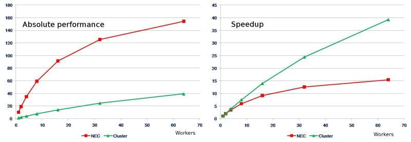
Stunt 1: When reporting perfomance data, it is never a good idea to report absolute performance! Rather, speedup (which is a relative measure) would be a better choice.

Stunt 1 on performance graphs: absolute performance Vs relative speedup

A better way of plotting performance data:

Efficiency-Time spectrum#

Why? People care about two observable properties:

Time until job completes.
Cost in core-hours or dollars to do job.

Most HPC applications have access to large machines, so don’t really care how many processes they use for any given job.

plot(exec_time(.99, ps), 1 ./ exec_cost(.99, ps), ylims = [0, 0.1], title = "Strong scaling: Efficiency Vs time", xlabel = "t", ylabel = "Efficiency", label = "")
scatter!(exec_time(.99, ps), 1 ./ exec_cost(.99, ps), seriescolor = :blue, label = "")

Principles:

The log scale is your friend!
Both axes have tangible quantities people care about
Bigger is better on the \(y\) axis, and more pushed to the left is better on the \(x\) axis.

Tip

Recommended reading: Fooling the masses with performance results on parallel computers

4. Weak Scaling#

Strong scaling is concerned with keeping the problem size \(n\) fixed, but parallel computers are also used to solve large problems. If we keep the amount of work per processor fixed, and vary the number of processors (and therefore the problem size) we are looking at weak scaling.

Following the same notation as above, we now have for serial performance:

\[ P^s_{\textrm{variable size}} = \frac{s + p}{T^s_{\textrm{fixed size}}} = 1 , \]

as \(N=1\).

For parallel performance (work over time):

\[ P^p_{\textrm{variable size}} = \frac{s + p N^{\alpha}}{T^p_{\textrm{fixed size}} (N)} = \frac{s + (1-s) N^{\alpha}}{s+ (1-s) N^{\alpha -1}} = S_{\textrm{variable size}}, \]

identical to application speedup.

In the special case of \(\alpha= 0\) (strong scaling), we recover Amdahl’s law again.

For values of \(\alpha\), \(0 < \alpha < 1\) and very large number of workers (CPU counts) \(N \gg 1\):

\[ S_{\textrm{variable size}} \rightarrow \frac{s + (1-s) N^\alpha}{s} = 1 + \frac{p}{s}N^\alpha , \]

which is linear in \(N^\alpha\). As a result, weak scaling allows us to cross the so-called Amdahl Barrier and get unlimited performance, even for small \(\alpha\).

The ideal case of \(\alpha = 1\) simplifies to:

\[ S_{\textrm{variable size}}(\alpha = 1) = s + (1-s)N , \qquad \leftarrow \textrm{Gustafson's Law}, \]

and in this case speedup is linear in \(N\), even for small \(N\). This is called Gustafson’s law, which put in other words it is

the theoretical “slowdown” of an already parallelized task if running on a serial machine.

ns = 10 .* ps

plot(ps, ns ./ exec_cost(.99, ps, n=ns, latency=1), xscale = :log10, label = "10 p")

ns = 100*ps

plot!(ps, ns ./ exec_cost(.99, ps, n=ns, latency=1), xscale = :log10, label = "100 p", title = "Weak scaling", xlabel = "# procs", ylabel = "efficiency")

pl = plot()
for w in exp10.(range(; start = log10(0.1), length = 20, stop = log10(1e3)))
    ns = w .* ps
    plot!(exec_time(0.99, ps, n=ns, latency=1), ns ./ exec_cost(0.99, ps, n=ns, latency=1), label="", xscale = :log10, ylims = [0, 1])
end
xlabel!("time")
ylabel!("efficiency")
title!("Weak scaling")
display(pl)